Riemannian Geometry Approach

Riemannian geometry is a branch of differential geometry that studies smooth manifolds, and curved spaces with peculiar geometries. In these spaces’ notions of angles, the shortest path between two points, distances, the center of mass of several points, etc., allow us to study the analytic properties of mathematical operators from a geometric perspective, making them accessible to intuition^[1]. Riemannian approaches represent EEG trials as covariance matrices^[2], symmetric positive definite matrices, and manipulate them with an appropriate Riemannian geometry. Classifiers based on such geometry are called RGCs.
The spatial covariance matrices of EEG signals are a natural choice since they contain spatial and power information.
Denoting by E\in\R^{n\times t} a given mean centred EEG recording epoch with n electrodes and t samples.
The spatial sample covariance matrix P is given by:

P=\frac{1}{t-1}EE^T \ \ \ (1)

SPD matrices lie in a Riemannian space with the following metric (local at P):

ds^2=\|P^{-\frac{1}{2}}dPP^{-\frac{1}{2}}\|^2_F \ \ \ (2)

The objective is to classify covariance matrices in their native space, so it is possible to consider a differential geometry framework for SPD matrices:
Geodesic between two SPD matrices (P₁ and P₂):

\gamma(t) =P^{\frac{1}{2}}_1(P^{-\frac{1}{2}}_1P_2P^{-\frac{1}{2}}_1)P^{\frac{1}{2}}_1,  \ t ∈ [0: 1] \ \ \ (3)

Distance between two SPD matrices (P₁ and P₂)

\delta_R(P_1, P_2) = \int_0^1{\gamma(t)dt} = \| k \log(P_1^{-1}P_2)\|_F \ \ \ (4)

Mean of K SPD matrices:

G(P_1, ..., P_k) = \argmin_{P \in P(n)}\sum_{j=1}^k{\delta^2_R (P, P_j)} \ \ \ (5)

Given a point P \in P(n), it is possible for every point P_i \in P(n) to identify a tangent vector,S_i \in Sx(n) such as S_i = \gamma(0), with \gamma(t) the geodesic between P and P_i

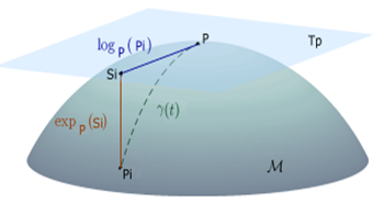
Fig 4: The complete set of tangent vectors define the Tangent Space, which is Euclidean.
Log map: S_i = \log_P(P_i) = P^{\frac{1}{2}} \log (P^{-\frac{1}{2}}P_iP^{-\frac{1}{2}})P^{\frac{1}{2}} \ \ \ (6)
Exp map: P_i = \exp_P(S_i) = P^{\frac{1}{2}} \log (P^{-\frac{1}{2}}S_iP^{-\frac{1}{2}})P^{\frac{1}{2}} \ \ \ (7)

Bibliography

Levi-Civita T. Lezioni di Calcolo Differenziale
Assoluto, Alberto Stock, Roma (1925) ↩︎Marco Congedo, Pedro Luiz Coelho Rodrigues, Christian Jutten. The Riemannian Minimum Distance
to Means Field Classifier. BCI 2019 - 8th International Brain-Computer Interface Conference, Sep
2019, Graz, Austria. ff10.3217/978-3-85125-682-6-02ff. ffhal-02315131 ↩︎