Pathfinding is the search for an optimal path from a start node to one or multiple goal nodes. The environment is usually represented as a weighted graph. Pathfinding algorithms are commonly used in robotics (agent navigation) and computer games (NPC navigation).
Dynamic pathfinding refers to pathfinding in dynamically changing or unknown environments. Changes or newly learned information about the environment are represented as changes in edge weights of the weighted graph.
Some of the well-known dynamic pathfinding algorithms are:
D* (Dynamic A*)
LPA* (Lifelong Planning A*)
D*-Lite
As their names suggest, these algorithms, just like many other pathfinding algorithms, are based on the A* algorithm. They all use a similar version of the priority queue used in A* and heuristics.
D* is an informed incremental search algorithm based on A* that has been developed as a path planning algorithm for partially known and dynamic environments. Different from A*, it keeps the values from previous searches and updates them if necessary. D* starts the search from the goal, and it can be implemented by moving agents.
D* is one of the first algorithms that can handle unknown environments, which made it a very important algorithm for this field of research. However, since the introduction of D*-Lite, the original D* is not being used as often.
D* formulates the problem space as a set of states denoting robot locations connected by directional arcs, each of which has an associated cost. These can also be referred to as nodes and directed edges with costs.
G: goal state or goal node
b(X)=Y: a backpointer from state X to a next state Y. Every state except for G has a backpointer. These repsesent paths to the goal.
c(X,Y): cost of the arc from a state X to state Y
OPEN: list for OPEN states, ordered by priority keys.
t(X): each state has a tag. t(X)=NEW means X has never been on the OPEN list; t(X)=OPEN means X is currently on the OPEN list and t(X)=CLOSE means X is no longer on the list.
h(G,X): heuristic value or path cost function. Returns the estimate of the sum of the arc costs from X to G.
k(G,X): key function. Defined to be the minimum of the h(G,X) value prior to modification and the set of all h(G,X) values assumed from the time it was placed on the list. The key function separates the states on the OPEN list into two. A state X is called a RAISE state if k(G,X)<h(G,X) and a LOWER state if k(G,X)=h(G,X). D* uses these two types of states to propagate information after a cost change.
D* iteratively selects and evaluates the node with the smallest key value from the OPEN list. It then updates all the neighboring nodes and places them into the OPEN list. After the search is complete, the cheapest path can be found by following the backpointers.
If the algorithm receives new information about a change or a newly discovered obstacle along the intended path, all the states affected by it get added into the OPEN list and marked as RAISE. Before a raised state increases in cost, D* checks if it can lower the cost of the state. If not, all the states that have a backpointer to the raised state are also marked as RAISE. These states also get evaluated and propagate RAISE the same way, creating a wave. If a raised state can be reduced, its backpointer gets updated and it passes LOWER to its neighbors.
Function: PROCESS-STATE()L1X←MIN-STATE()L2if X=NULL then return −1L3kold←GET-KMIN();DELETE(X)L4if kold<h(X) thenL5for each neighbor Y of X:L6if h(Y)≤koldandh(X)>h(Y)+c(Y,X) thenL7b(X)←Y;h(X)←h(Y)+c(Y,X)L8if kold=h(X) thenL9for each neighbor Y of X:L10if t(Y)=NEWorL11(b(Y)=Xandh(Y)=h(X)+c(X,Y))orL12(b(Y)=Xandh(Y)>h(X)+c(X,Y)) thenL13b(Y)←X;INSERT(Y,h(X)+c(X,Y))L14elseL15for each neighbor Y of X:L16if t(Y)=NEWorL17(b(Y)=Xandh(Y)=h(X)+c(X,Y)) thenL18b(Y)←X;INSERT(Y,h(X)+c(X,Y))L19elseL20if b(Y)=Xandh(Y)>h(X)+c(X,Y) thenL21INSERT(X,h(X))L22elseL23if b(Y)=Xandh(X)>h(Y)+c(Y,X)L24and t(Y)=CLOSEDandh(Y)>kold thenL25INSERT(Y,h(Y))L26return GET-KMIN()
Function: MODIFY-COST(X,Y,cval)L1c(X,Y)←cvalL2if t(X)=CLOSED then INSERT(X,h(X))L3return GET-KMIN()
LPA* is another incremental dynamic pathfinding algorithm that finds the shortest path between a start node and a goal node. It generalizes both DynamicSWSF-FP and A* to reduce the planning time and can be considered the incremental version of A*. Instead of recalculating every g-value after an update to the graph, it reuses the values from previous searches and updates the g-values if necessary. LPA* starts the search from the start node, and start and goal nodes are fixed, so the start node doesn’t get updated if the agent changes position.
Succ(s): returns the set of successors of vertex s.
Pred(s): returns the set of predecessors of vertex s.
c(s,s′): stands for the cost of moving from vertex s to vertex s′.
h(s,sgoal): heuristic value from node s to goal node. Usually corresponds to the cost of the shortest/cheapest path from node s to goal node if there were no obstacles. It shouldn't return a negative value and must obey the triangle inequality.
g(s): shortest distance from node s to start, corresponds to the g-values of A*.
rhs(s): one-step lookahead value for g-value. Any potential update for a g-value first gets written here. Always satisfies the following relationship for any vertex s:
k(s): key value. Represented as a vector with 2 components: k(s)=[k1(s);k2(s)], where k1(s)=min(g(s),rhs(s))+h(s,sgoal) and k2(s)=min(g(s),rhs(s)). Keys are compared according to a lexicographic ordering. k1(s) corresponds directly to the f-values of A* and k1(s) corresponds to the g-values of A*.
The paper introduces the term inconsistency, which means the g and rhs values for a vertex are not the same. An inconsistent vertex is called overconsistent if and only if g(s)>rhs(s), or underconsistent if and only if g(s)<rhs(s). The algorithm depends on the resolution of inconsistencies.
LPA* algorithm consists of 4 functions and one main loop. These are:
CalculateKey(s): returns the key k(s) for a given vertex s. The vertices in the queue are sorted according to key value.
Initialize(): sets all the g and rhs values to ∞ for all vertices. After that sets the rhs value of the start node to 0 and inserts it into the queue U.
UpdateVertex(u): updates the rhs value of the vertex u, if u is not the start node, by the sum of the g value of a predecessor s′ and the cost of the edge between them. Vertex s′ is the predecessor that minimizes this sum. Removes the old u from the queue and adds it again if the vertex is still inconsistent. This results in the queue consisting of inconsistent vertices only.
ComputeShortestPath(): ComputeShortestPath(): this is the actual search function. As long as the goal node is inconsistent or there is at least one vertex in the queue with a key value less than the key value of the goal, the vertex with the highest priority gets checked for inconsistency.
If it's overconsistent, g-value gets the same value as the rhs-value and all the successor vertices get updated accordingly.
If it's underconsistent, g-value gets set to ∞ and this vertex and all the successor vertices get updated accordingly.
Main Loop: after initialization, it enters an infinite loop that completes a search and updates the graph if there are any changes in each iteration.
procedure CalculateKey(s){01}return [min(g(s),rhs(s))+h(s,sgoal);min(g(s),rhs(s))];procedure Initialize(){02}U←∅;{03}for all s∈S:rhs(s)=g(s)=∞;{04}rhs(sstart)=0;{05}U.Insert(sstart,CalculateKey(sstart));procedure UpdateVertex(u){06}if (u=sstart):rhs(u)=s′∈Pred(u)min(g(s′)+c(s′,u));{07}if (u∈U):U.Remove(u);{08}if (g(u)=rhs(u)):U.Insert(u,CalculateKey(u));procedure ComputeShortestPath(){09}while (U.TopKey()<CalculateKey(sgoal)orrhs(sgoal)=g(sgoal)){10}u←U.Pop();{11}if (g(u)>rhs(u)){12}g(u)←rhs(u);{13}for all s∈Succ(u):UpdateVertex(s);{14}else{15}g(u)←∞;{16}for all s∈Succ(u)∪{u}:UpdateVertex(s);procedure Main(){17}Initialize();{18}forever{19}ComputeShortestPath();{20}wait for changes in edge costs;{21}for all directed edges (u,v) with changed costs{22}Update the edge cost c(u,v);{23}UpdateVertex(v);
The paper shows that compared to A*, LPA* needs significantly fewer vertex expansions, vertex accesses, and heap percolates in a dynamic environment. The experiment used fifty randomly generated eight-connected grid worlds of size 40×40 with an obstacle density of 40. After 500 changes to the grid worlds, the results in Table 1 were obtained.
D*-Lite is a dynamic pathfinding algorithm that is based on LPA*. D*-Lite is algorithmically different from D*; however, it implements the same behavior. Since it is a simpler algorithm than D*, it is called Lite.
D*-Lite is one of the most important pathfinding algorithms, since it is very efficient in most cases and easy to understand and extend. Because of this, many D*-Lite variants such as Field D* and Anytime D* have been created. Even though it is an older algorithm, D*-Lite is still commonly used in game development.
Even though LPA* is a good algorithm for pathfinding, because of fixed start and goal nodes, it cannot be implemented with a moving agent. On the other hand, D*-Lite can be used with a dynamically changing start node and a fixed goal node.
As a result of the dynamically changing start node, the main loop of D*-Lite terminates as soon as the goal node is reached. As its name suggests, the main loop of LPA* runs forever.
The direction of the search is also different between D*-Lite and LPA*. Just like D*, D*-Lite also starts the search from the goal node.
D*-Lite introduces a new variable km. This represents the sum of all the heuristic value between the old and new agent positions after each move. km is used by the k1 values of the keys. D*-Lite defines the key value for a vertex s as follows: k(s)=[k1(s);k2(s)], where k1(s)=min(g(s),rhs(s))+h(sstart,s)+km and k2(s)=min(g(s),rhs(s)). All of the other variables and functions remain the same.
The algorithm remains essentially the same as in LPA*, however, as a result of starting from the end node, all the Succ() function calls get replaced with Pred(), and all the Pred() function calls get replaced with Succ() in the pseudocode. Similarly, all usages of the start node sstart are replaced with the goal node sgoal, and all usages of the goal node sgoal are replaced with the start node sstart.
Other than these changes, the functionality of CalculateKey(s), Initialize() and UpdateVertex(s) remain the same.
ComputerShortestPath() also keeps it functionality, however, now before evaluating inconsistencies, it makes sure that all the vertices being evaluated doesn't have a more optimistic key from the previous searches. If so, it recalculates the key and the vertex is added into the queue again. After a change in the graph, the vertices in the queue are not necessarily updated, so the change in the km value might worsen their key values. This is why these new lines are necessary.
Unlike other functions, the main loop gets a more significant update. First Initialize() and ComputerShortestPath() get called and then a loop starts that runs until the goal node is reached. The loop functions as follows:
The agent moves to the next vertex of the previously calculated cheapest path. It checks for changes in the environment.
If there are changes, km value is calculated as follows: km=km+h(slast,sstart) where s_{last} is the position/vertex of the agent after the last change and s_{start} is the current position/vertex. After this, the graph gets updated accordingly and ComputerShortestPath() gets called again to find the new cheapest path.
procedure CalculateKey(s){01′}return [min(g(s),rhs(s))+h(sstart,s)+km;min(g(s),rhs(s))];procedure Initialize(){02′}U←∅;{03′}km←0;{04′}for all s∈S:rhs(s)=g(s)=∞;{05′}rhs(sgoal)←0;{06′}U.Insert(sgoal,CalculateKey(sgoal));procedure UpdateVertex(u){07′}if (u=sgoal):rhs(u)=s′∈Succ(u)min(c(u,s′)+g(s′));{08′}if (u∈U):U.Remove(u);{09′}if (g(u)=rhs(u)):U.Insert(u,CalculateKey(u));procedure ComputeShortestPath(){10′}while (U.TopKey()<CalculateKey(sstart)orrhs(sstart)=g(sstart)){11′}kold←U.TopKey();{12′}u←U.Pop();{13′}if (kold<CalculateKey(u)){14′}U.Insert(u,CalculateKey(u));{15′}else if (g(u)>rhs(u)){16′}g(u)←rhs(u);{17′}for all s∈Pred(u):UpdateVertex(s);{18′}else{19′}g(u)←∞;{20′}for all s∈Pred(u)∪{u}:UpdateVertex(s);procedure Main(){21′}slast←sstart;{22′}Initialize();{23′}ComputeShortestPath();{24′}while (sstart=sgoal){25′}/* if g(sstart)=∞ then no known path */{26′}sstart←args′∈Succ(sstart)min(c(sstart,s′)+g(s′));{27′}Move to sstart;{28′}Scan graph for changed edge costs;{29′}if any edge costs changed{30′}km←km+h(slast,sstart);{31′}slast←sstart;{32′}for all directed edges (u,v) with changed costs{33′}Update c(u,v);{34′}UpdateVertex(u);{35′}ComputeShortestPath();
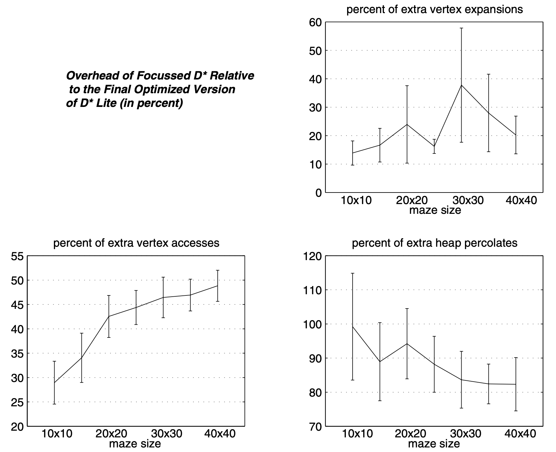
The paper found that D*-Lite is at least as efficient as D* and ran an experiment comparing Focused D*, an improved version of D*, and an optimized version of D*-Lite for goal-directed navigation in unknown terrain. They used randomly generated 50 terrains, which were discretized into cells with uniform resolution, for each of the seven sizes whose obstacle density varies from 10 to 40 percent. The following graphs show the percentages of extra vertex expansions, extra vertex accesses and extra heap percolates needed by D* compared to D*-Lite:
Figure 2: Overhead of Focussed D* Relative to the Final Optimized Version of D* Lite (in percent)
Stentz, Anthony. "Optimal and efficient path planning for partially-known environments." Proceedings of the 1994 IEEE international conference on robotics and automation. IEEE, 1994. pdf↩︎↩︎
Koenig, Sven, and Maxim Likhachev. "Incremental a." Advances in neural information processing systems 14 (2001). pdf↩︎↩︎↩︎
Koenig, Sven, and Maxim Likhachev. "D* lite." Eighteenth national conference on Artificial intelligence. 2002. pdf↩︎↩︎↩︎