Modern Machine-Learning Algorithms: For Classifying Cognitive and Affective States from EEG Signals

This article is basen on the paper of A. Appriou, A. Cichocki and F. Lotte, "Modern Machine-Learning Algorithms: For Classifying Cognitive and Affective States From Electroencephalography Signals,"
Considering the problem of classification accuracies, cognitive or affective state estimation from brain signals is one of the main difficulties in creating a passive brain-computer interface application. This article proposes a study and a comparison of recent Machine-Learning algorithms, notably Riemannian-geometry-based and CNN classifiers for cognitive and affective classification.

Experiment

Mental workload Data Set

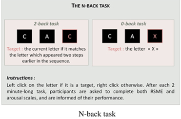
Fig.1: The N-back task requires responses to target and non-target characters.

The data set is made by 28 EEG signals, active in a 10/20 system without T7, T8, Fp1, and Fp2, recorded from 22 users^[1]. The study is composed of both subject-specific and subject-independent. For the calibration for subject-independent, the training set comprised all trials of all users except the current user, i.e., around 21 × 1,440 = 30,240 training trials. For the latter, the first half of each user’s trial is used for training and the second half for testing.

To induce mental workload variations, N-back tasks are used: the user had to indicate whether a letter displayed on the screen was the same as the one displayed N letters before, in a stream of successively displayed letters. Here, 2-s trials from a 0-back task were labeled low workload while those from a 2-back were labeled high workload. In total, 720 trials were available for each workload level and user.^[2]

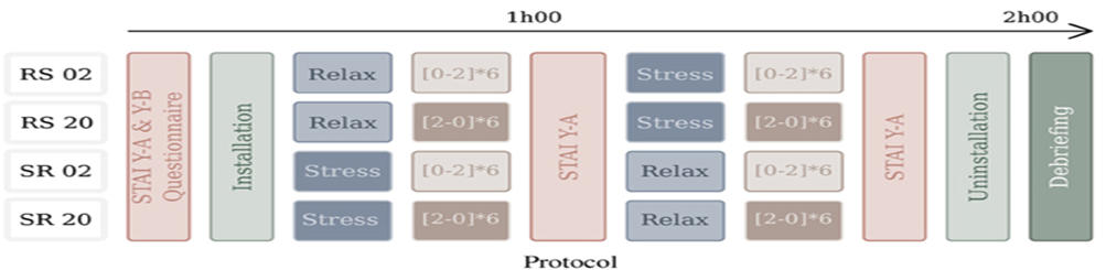
Fig.2: The experimental protocol
The experimental protocol is based on four scenarios, composed of the combination of two workload tasks, 0-back (easy) and 2-back (difficult)

Emotion EEG Data Set

The clustering of emotion dimension is modeled by the Circumplex Model of Russell, which localized any affective state on a 2D plane. The first axes is the valence varying from a positive to a negative feeling, the second is arousal varying from calm to excited.^[3]

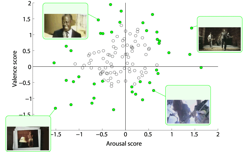
Fig.3: value for the ratings of each video in the assessment. Videos selected for use in the experiment are highlighted in green.

It used music-video clips to influence two types of emotion dimensions, valence, and arousal. The data set contains 40 trials, corresponding to 40 music-video clips, recorded on 32 participants. EEGs were recorded using 32 electrodes (placed according to the international 10–20 system). Valence and arousal levels were measured using Russell’s valence-arousal scale directly after each video by clicking on a 1 to 9 continuous scale. This self-assessment system on a continuous scale makes the classes definition more complex:^[4].

Riemannian Geometry Approach

Riemannian geometry is a branch of differential geometry that studies smooth manifolds, and curved spaces with peculiar geometries. In these spaces’ notions of angles, the shortest path between two points, distances, the center of mass of several points, etc., allow us to study the analytic properties of mathematical operators from a geometric perspective, making them accessible to intuition^[5]. Riemannian approaches represent EEG trials as covariance matrices, symmetric positive definite matrices, and manipulate them with an appropriate Riemannian geometry. Classifiers based on such geometry are called RGCs.
The spatial covariance matrices of EEG signals are a natural choice since they contain spatial and power information.
Denoting by E\in\R^{n \times t} a given mean centred EEG recording epoch with n electrodes and t samples.
There are already methods such as FgMDM and TSC who present promising result, therefore in the next section is presented new variation of those methods who has proven to perform better result.

New Methods

FBFgMDM

Contrary to FgMDM, which exploits EEG signals in a single frequency band, FBFgMDM applies FgMDM in multiple bands separately and combines the resulting distances to exploit additional spectral information. This approach should improve classification performances, as FBCSP did to improve CSP. To do so, FBFgMDM first filters EEG signals in multiple bands using a filter bank, as for FBCSP. Here is used the same bands as the FBCSP, i.e., 4–8 Hz, 8–12 Hz, …, 36–40 Hz. Then, for the EEG signals in each frequency band j, this method first uses a regular FgMDM, i.e., it computes the Riemannian distances \delta _2(P_{kj},P_{ij}) between a geodesic filtered SPD matrix P^{ij} and each class centroid P_{kj}. Then, from all nine bands j, the four that are most useful for classification are selected with mRMR feature selection^[6] on the Riemannian distances \delta _2(P_{kj},P_{ij}) used as features, on the training set. For testing, it's possible to compute the squared Riemannian distances for the four bands selected using mRMR only and sum them as

\gamma_2(P_k,P_i)=\sum_{j\in\Omega}\delta_2(G_{kj},C_{ij}) \ \ \ (10)

where \Omega is the set of frequency bands selected with mRMR. there are now obtained k new distances \gamma_2(P_k,P_i) to each class k for each trial i. The classification prediction results in choosing the class y_i for which the summed squared distance to the centroid is the smallest, i.e., 

y_i=\argmin_k(\gamma_2(P_k,P_i)) \ \ \ (11)

FBTSC

FBTSC also exploits more spectral information than TSC, by using a filter bank, projecting matrices P{ij}, bandpass filtered in bands 4–8 Hz, 8–12 Hz, …, 36–40 Hz to the tangent space using (4). Then, the probabilities that the vectorized upper-triangular elements of the projected SPD matrix S_{ij} belongs to class k is calculated using standard classification algorithms with probabilistic outputs, such as LDA or LR. Here, it has been used LR, which directly provides such probability with its softmax function. Since it has been done so for nine frequency bands, in two classes k, now are available nine pairs of probabilities. From these pairs, the four most relevant are selected using mRMR on the training set. Finally, multipling the probabilities associated with each class k, for the selected bands only, to end up with two probabilities, using

\bar{P}_{ki}= \prod{P_{kij}} \ \ \ (12)

where \bar{P}_{ki} is the probability of trial i being part of class k, and P_{kij} is the probability of a projected SPD matrix S_{ij}, bandpass filtered in frequency band j, to be part of class k. The classification prediction results in choosing the class yi for which \bar{P}_{ki} is the highest,i.e.

y_i= \argmax_k(\bar{P}_{ki})  \ \ \ (13)

Result

Here is presented the resuls related for each experiment performed by the following algorithms: classical one (CSP, FBCSP), Riemannian Geometry based (FgMDM, TSC, FBFgMDM, FBTSC) and CNN.

Workload Study Results

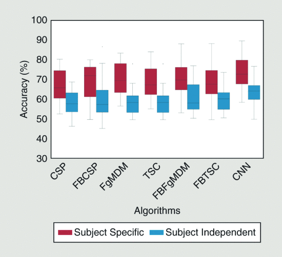
Fig.4: workload result
Is performed a two-way ANOVA with repeated measures to evaluate the performances of factor Algorithm according to factor
Calibration Type (subject-specific versus subject-independent studies). It revealed a main effect of Algorithm
GG(1,22) = 0.517, p = 0.001, and Calibration Type F(1,22)
= 33-308, p ≤ 0.0001, but not for Calibration
Type*Algorithm GG(1,22) = 0.558, p = 0.618.
The best resuslt both in subject-specific and subject-indipendent is obtained by CNN, and the new algorithms provide the second best performance. The worst result has been done by the classical method CSP + LDA

Affective State Estimation Results

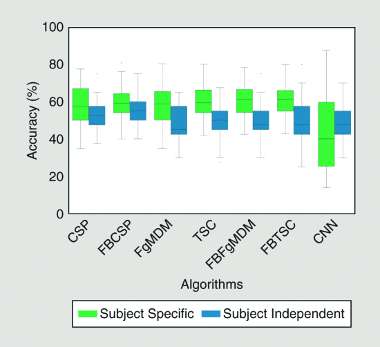
Fig.5: emotion–valence result

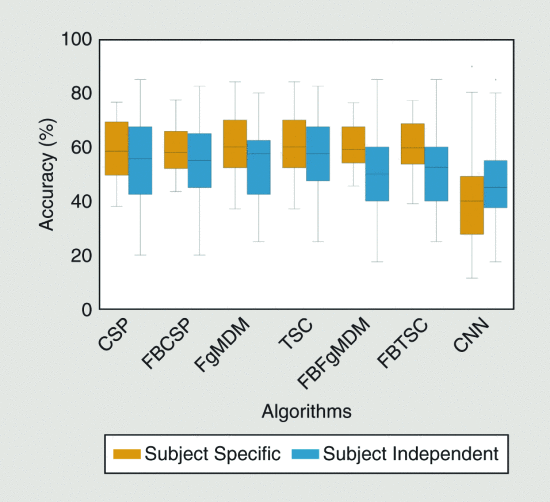
Fig.6: emotion–arousal result
In the figure is presented the performance for valence and arousal.
They show significant differences in the subject-specific calibration.
The best performance is made by GRC's algorithms, in particular FBFgMDM, FBTSC.
The wrost in both calibration the CNN shows the worst result.

Bibliography

C. Mühl, C. Jeunet, and F. Lotte, “EEG-based workload estimation across affective
contexts,” Front. Neurosci., vol. 8, pp. 1–15, June 2014. doi: 10.3389/fnins.2014.00114. ↩︎M. Clerc, L. Bougrain, and F. Lotte, Brain-Computer Interfaces 1: Methods and
Perspectives. Hoboken, NJ: Wiley, 2016. ↩︎J. A. Russell, “A circumplex model of affect,” J. Pers. Soc. Psychol., vol. 39, no. 6,
pp. 1161–1178, 1980. doi: 10.1037/h0077714 ↩︎S. Koelstra et al., “DEAP: A database for emotion analysis using physiological signals,” IEEE Trans. Affective Comput., vol. 3, no. 1, pp. 18–31, 2012. doi:
10.1109/T-AFFC.2011.15. ↩︎Levi-Civita T. Lezioni di Calcolo Differenziale
Assoluto, Alberto Stock, Roma (1925) ↩︎H. Peng, F. Long, and C. Ding, “Feature selection based on mutual information:
Criteria of max-dependency, max-relevance, and min-redundancy,” IEEE Trans. Pattern
Anal. Mach. Intell., vol. 27, no. 8, pp. 1226–1238, 2005. doi: 10.1109/TPAMI.2005.159. ↩︎